Empirical Data

GARCH-based Asymmetric Least Squares Risk Measures

Distribution of risk measures

• We calculate the quantiles, expectiles and extremiles from the standard residuals:

  • First, we compute the risk measures via QMLE at \(\tau =\{1\%,5\%,10\%\}\).

  • Second, we compute the risk measures via (QMLE) bootstrap at \(\tau =\{1\%,5\%,10\%\}\).

Empirical Data

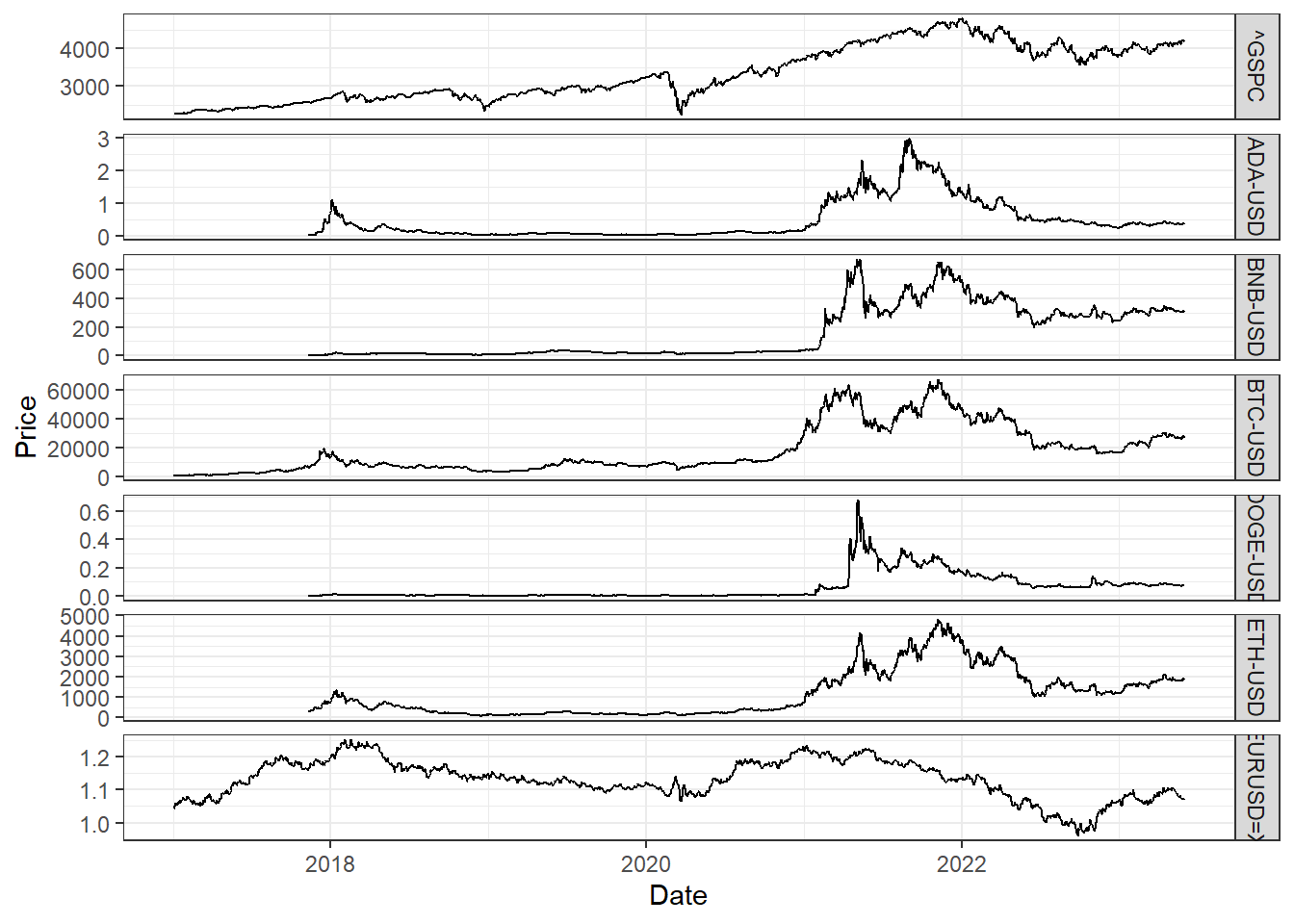
We collect the daily price data of S\&P 500, EUR/USD, BTC/USD, ETH-USD, BNB-USD, DOGE-USD and ADA-USD

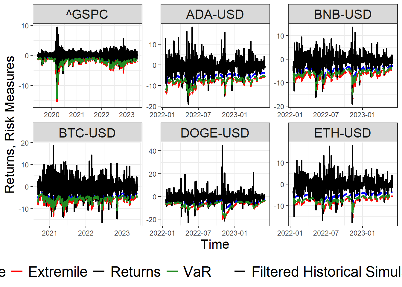
The following dashboard summarizes all risk measures considering Historical, Parametric and Filtered Historical Simulation.

Figure below show the Filtered Historical Simulation risk measures for several assets for \(\tau = 0.05\).

risk.data = 
  readRDS('C:/Users/Olive/Documents/Github/Thesis/GARCH-Based Asymetric Least Squares for Financial Time Series/Dashboards/GARCH-Based  ALS Empirical Analysis/empirical/risk.data.RDS')


risk.data %>%
  filter(window %in% c('expanding')) %>% 
  filter(type %in% c('Filtered Historical Simulation','Returns')) %>%
  filter(measure %in% c('VaR','Returns','Expectile','Extremile')) %>%
  filter(level %in% 0.05) %>% 
  filter(!(ticker %in% c('EURUSD=X'))) %>% 
  ggplot() +
  geom_line(aes(x = date, y = estimate, color = measure, linetype = type), linewidth = 1) +
  scale_color_manual(values = 
                       c('Returns' = 'black' ,
                         'Extremile' = 'red',
                         'Expectile' = 'blue',
                         'VaR' = 'forestgreen',
                         'Expected Shortfall' = 'purple')) +
  scale_linetype_manual(
    values = c('Returns' = 'solid',
               'Filtered Historical Simulation' = 'longdash')) +
  theme_bw() +
  labs(x = 'Time', y = 'Returns, Risk Measures') +
  facet_wrap(~ticker, scales = 'free') + 
  theme(legend.title = element_blank(),
            legend.position = 'bottom',
            legend.text = element_text(size = 18),
            axis.title = element_text(size = 16),
            strip.text = element_text(size = 16))

Bootstrap Confidence Interval

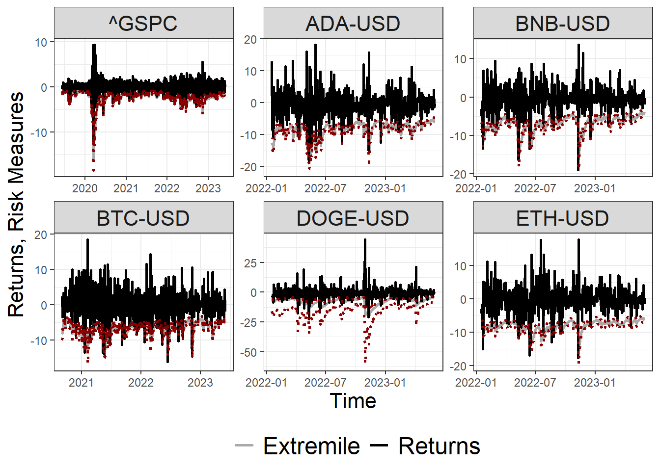
The following dashboard reports the bootstrap confidence interval of all Filtered Historical Simulation risk measures.

Figure below shows the bootstrap confidence interval of the \(\tau\)-th Extremile (\(\tau =0.05\)) risk measure considering a bootstrap confidence level of \(\alpha = 0.05\).

ci.data = 
  readRDS('C:/Users/Olive/Documents/Github/Thesis/GARCH-Based Asymetric Least Squares for Financial Time Series/Dashboards/GARCH-Based  ALS Empirical Analysis/empirical_ci/ci.data.RDS')


ci.data %>%
  filter(window %in% c('expand')) %>% 
  filter(measure %in% c('Returns','Extremile')) %>%
  filter(level %in% 0.05) %>% 
  filter(!(ticker %in% c('EURUSD=X'))) %>% 
  fill(c(lower_bound,upper_bound)) %>% 
  ggplot() +
  geom_line(aes(x = date, y = estimate, color = measure), linetype = 'solid', linewidth = 1) +
  geom_line(aes(x = date, y = upper_bound), linetype = 'dotted', color = 'darkred',linewidth = 1) +
  geom_line(aes(x = date, y = lower_bound), linetype = 'dotted', color = 'darkred', linewidth = 1) +
  scale_color_manual(
    values = c('Returns' = 'black' ,
               'Extremile' = 'darkgrey',
               'Expectile' = 'blue',
               'VaR' = 'forestgreen')) + 
  labs(x = 'Time', y = 'Returns, Risk Measures') +
  theme_bw() +
  facet_wrap(~ticker, scales = 'free') +
  theme(legend.title = element_blank(),
            legend.position = 'bottom',
            legend.text = element_text(size = 18),
            axis.title = element_text(size = 16),
            strip.text = element_text(size = 16))

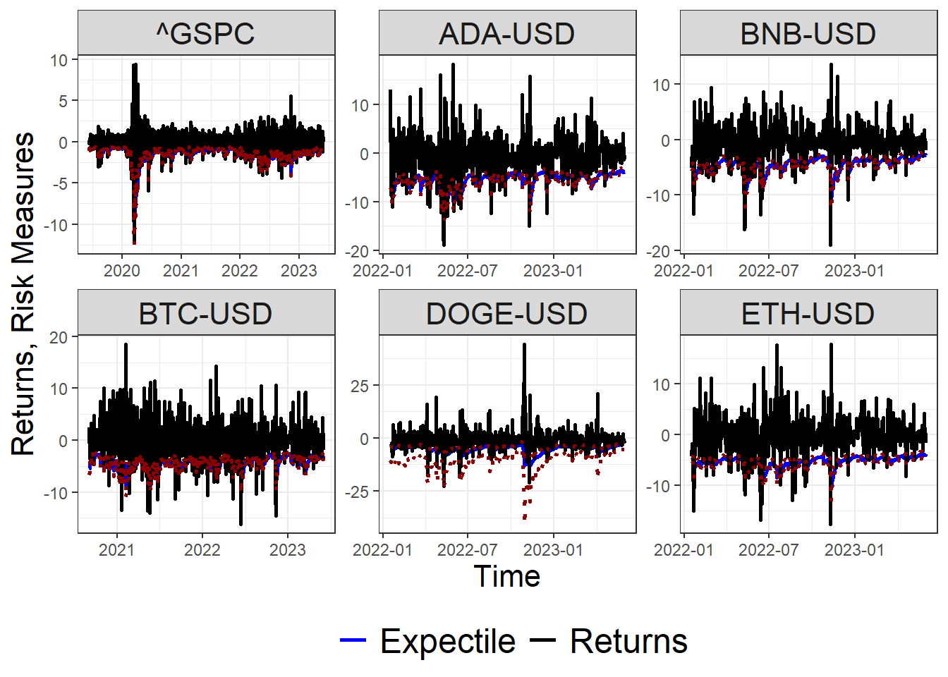
Likewise, Figure below shows the bootstrap confidence interval of the \(\tau\)-th Expectile (\(\tau =0.05\)) risk measure considering a bootstrap confidence level of \(\alpha = 0.05\).

ci.data %>%
  filter(window %in% c('expand')) %>% 
  filter(measure %in% c('Returns','Expectile')) %>%
  filter(level %in% 0.05) %>% 
  filter(!(ticker %in% c('EURUSD=X'))) %>% 
  fill(c(lower_bound,upper_bound)) %>% 
  ggplot() +
  geom_line(aes(x = date, y = estimate, color = measure), linetype = 'solid', linewidth = 1) +
  geom_line(aes(x = date, y = upper_bound), linetype = 'dotted', color = 'darkred',linewidth = 1) +
  geom_line(aes(x = date, y = lower_bound), linetype = 'dotted', color = 'darkred', linewidth = 1) +
  scale_color_manual(
    values = c('Returns' = 'black' ,
               'Extremile' = 'darkgrey',
               'Expectile' = 'blue',
               'VaR' = 'forestgreen')) + 
  labs(x = 'Time', y = 'Returns, Risk Measures') +
  theme_bw() +
  facet_wrap(~ticker, scales = 'free') +
  theme(legend.title = element_blank(),
            legend.position = 'bottom',
            legend.text = element_text(size = 18),
            axis.title = element_text(size = 16),
            strip.text = element_text(size = 16))

Drawdown

equity_ticker <- c('^GSPC','EURUSD=X','BTC-USD',
                   'ETH-USD','BNB-USD','DOGE-USD','ADA-USD')

start_date <- ymd("2017-01-01")

end_date <- ymd("2023-06-01")

data <- 
  yf_get(equity_ticker,start_date,end_date) %>%
  select(ref_date,ticker,price_adjusted,ret_adjusted_prices) %>%
  rename_with(~ c('date','ticker','price','returns')) %>%
  drop_na() %>%
  group_by(ticker) %>%
  ungroup()

Cryptocurrencies reached their peak values during the market’s surge in late 2021. However, many digital assets experienced significant price corrections in the following year. In particular, Bitcoin reached its record-breaking all-time high of \(\$67,566.83\) on November 8, 2021, although experienced a substantial decline in value, trading at \(\$15,787.28\) on November 21, 2022.

data %>% 
  ggplot() +
  geom_line(aes(x = date, y = price)) +
  labs(x = 'Date', y = 'Price') + 
  facet_grid(ticker ~ ., scales = 'free') +
  theme_bw()

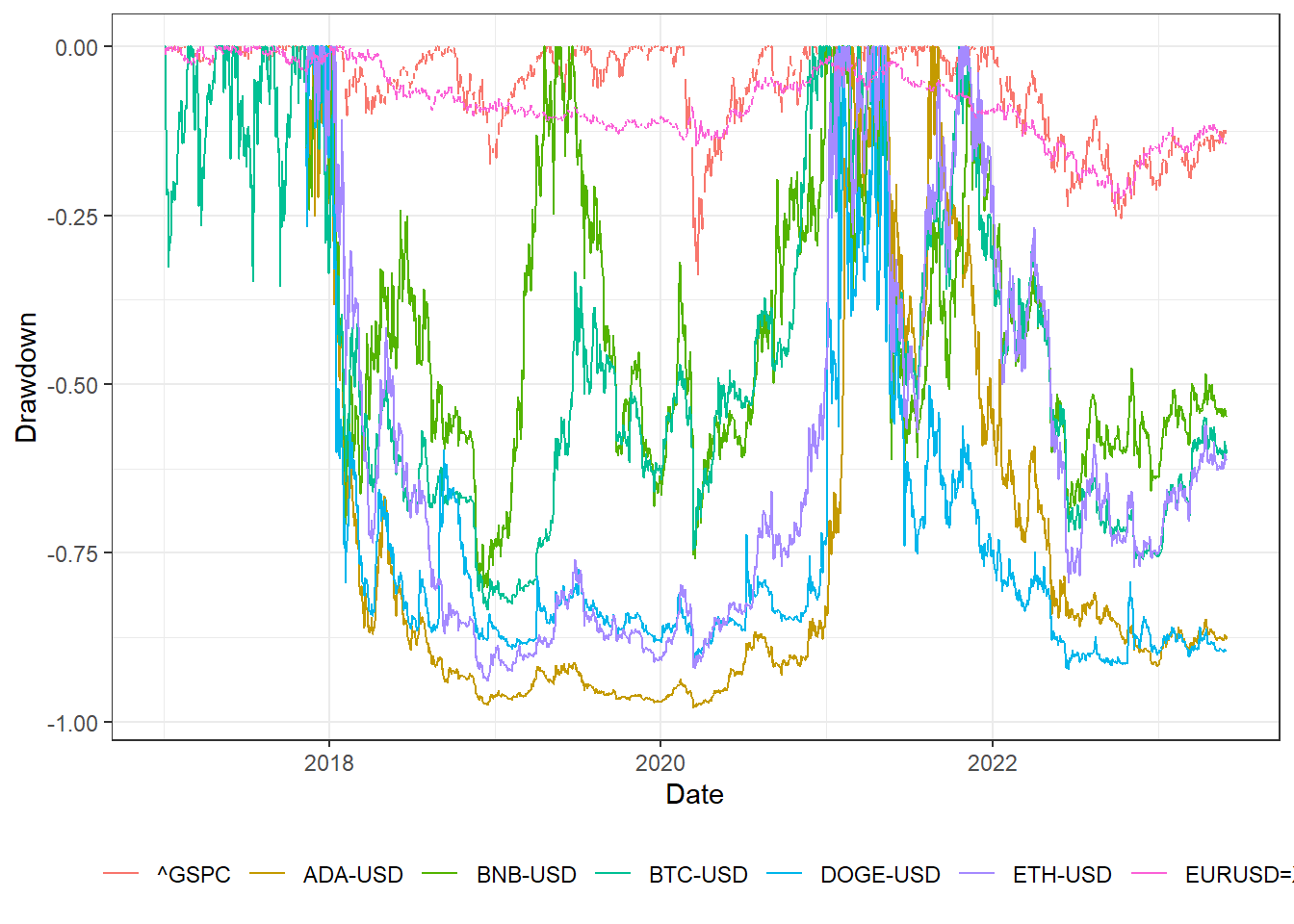
The figure below presents a comparative analysis of historical drawdowns among various cryptocurrencies, namely Bitcoin (BTC-USD), Bitcoin Cash (BTC/USD), Ethereum (ETH-USD), Binance Coin (BNB-USD), Dogecoin (DOGE-USD), and Cardano (ADA-USD), with respect to the S&P 500 and EUR/USD. It is evident that Cardano, Ethereum, Dogecoin, Bitcoin, and Binance Coin have experienced significant declines, surpassing 80% since reaching their respective peak values. In contrast, the drawdowns observed in the S&P 500 and EUR/USD have been relatively milder, hovering around 30%. These results show the substantial price fluctuations and volatility observed within the cryptocurrency market while highlighting the comparatively more stable performance of traditional financial benchmarks like the S&P 500 and EUR/USD.

data %>% 
  pivot_wider(id_cols = date, names_from = ticker, values_from = returns)  %>%
  as.xts() %>% 
  Drawdowns() %>%
  as.data.frame() %>% 
  rownames_to_column(var = 'date') %>% 
  mutate(date = as_date(date)) %>% 
  pivot_longer(-date, names_to = 'ticker', values_to = 'drawdown') %>% 
  ggplot() +
  geom_line(aes(x = date, y = drawdown, color = ticker)) +
  theme_bw() +
  labs(x = 'Date', y = 'Drawdown') + 
  theme(legend.position = 'bottom',
        legend.title = element_blank()) +
   guides(col = guide_legend(nrow = 1))

Codes for replication

QMLE.bootstrap <- function(fit, data, n.bootfit = 999, n.ahead = 1, tau = 0.05, alpha = 0.05){
  
  # initial paarameters
  
  n.bootpred = n.ahead 
  
  N = length(data)
  
  set.seed(1)
  
  # ---------------------------------------
  
  # generate paths of equal length to data based on empirical re-sampling of z
  # Pascual, Romo and Ruiz (2006) p.2296 equation (5)
  
  fz = as.numeric(residuals(fit))
  
  empz = matrix(0, ncol = n.bootfit, nrow = N)
  
  empz = apply(as.data.frame(1:n.bootfit), 1, FUN=function(i){
    
    sample(fz, N, replace = TRUE)
    
  })
  
  # presigma uses the same starting values as the original fit
  # in paper they use alternatively the unconditional long run sigma 
  # Pascual, Romo and Ruiz (2006) p.2296 equation (5) (P.2296 paragraph 2  "...marginal variance..."
  
  coef = as.numeric(coef(fit))
  
  spec =  
    ugarchspec(
      mean.model = list(armaOrder = c(0, 0), include.mean = FALSE),
      variance.model = list(model = 'sGARCH', garchOrder = c(1,1)),  
      fixed.pars = list(
        mu = 0, # our mu (intercept)
        ar1 = 0, # our phi_1 (AR(1) parameter of mu_t)
        ma1 = 0, # our theta_1 (MA(1) parameter of mu_t)
        omega = coef[1], # our alpha_0 (intercept)
        alpha1 = coef[2], # our alpha_1 (ARCH(1) parameter of sigma_t^2)
        beta1 = coef[3])) # our beta_1 (GARCH(1) parameter of sigma_t^2)
  
  presigma = tail(sqrt(fitted(fit)),1)
  
  prereturns = tail(data, 1)
  
  preresiduals = tail(fz, 1) 
  
  paths = ugarchpath(spec, 
                     n.sim = N, 
                     m.sim = n.bootfit, 
                     presigma = presigma,
                     prereturns = prereturns,
                     preresiduals = preresiduals,
                     n.start = 0, 
                     custom.dist = list(name = "sample", distfit = as.matrix(empz)))
  
  fitlist = vector(mode="list", length = n.bootfit)
  
  simseries = fitted(paths)
  
  nx = NCOL(simseries)
  
  # generate path based forecast values
  # for each path we generate n.bootpred vectors of resampled data of length n.ahead
  # Equation (6) in the PRR paper (again using z from original fit)
  #-------------------------------------------------------------------------
  
  fitlist = lapply(as.list(1:nx), FUN = function(i){
    
    fit.boot = garchx(y = as.numeric(simseries[,i]), order = c(1,1))
    
    theta = coef(fit.boot)
    
    df = tibble('ID' = i,
                'omega' = theta[1],
                'alpha' = theta[2], 
                'beta' = theta[3],
                'epsilon' = data[length(data):1],
                'eta' = c(as.numeric(residuals(fit.boot)),NA), 
                'j' = seq(0,length(data)-1,1),
                'sum' = beta^j*(lead(epsilon)^2 - omega/(1-alpha-beta))) %>% 
      drop_na() %>% 
      reframe(
        ID = unique(ID),
        omega = unique(omega),
        alpha = unique(alpha),
        beta = unique(beta),
        epsilon = first(epsilon), 
        sum = sum(sum),
        sigma2.hat = omega + alpha*epsilon^2 + beta*(omega/(1-alpha - beta) + alpha*sum),
        extremile.hat = sqrt(sigma2.hat)*extremile(eta, probs = tau),
        expectile.hat = sqrt(sigma2.hat)*expectile(eta, probs = tau),
        VaR.hat = sqrt(sigma2.hat)*quantile(eta, probs = tau),
        ES.hat = sqrt(sigma2.hat)*mean(if_else(eta < quantile(eta, probs = tau),eta,NA),na.rm = TRUE))
    
    return(df)
    
  })
  
  confidence.interval = 
    fitlist %>% 
    bind_rows() %>% 
    select(ID,contains('hat')) %>% 
    pivot_longer(-ID, names_to = 'measure', values_to = 'estimate') %>% 
    group_by(measure) %>% 
    summarise_at(vars(estimate), 
                 .funs = list(lower_bound = ~ quantile(., probs = alpha/2),
                              upper_bound = ~ quantile(., probs = 1-alpha/2))) %>% 
    left_join(
      tibble(eta = as.numeric(residuals(fit)),
             sigma2.hat = as.numeric(predict(fit,n.ahead = 1))) %>%
        reframe(
          ID = 1,
          sigma2.hat = unique(sigma2.hat),
          extremile.hat = sqrt(sigma2.hat)*extremile(eta, probs = tau),
          expectile.hat = sqrt(sigma2.hat)*expectile(eta, probs = tau),
          VaR.hat = sqrt(sigma2.hat)*quantile(eta, probs = tau),
          ES.hat = sqrt(sigma2.hat)*mean(if_else(eta < quantile(eta, probs = tau),eta,NA),na.rm = TRUE)) %>% 
        pivot_longer(-ID,names_to = 'measure', values_to = 'estimate') %>% 
        select(-ID)) %>% 
    relocate(measure,lower_bound,estimate,upper_bound)
  
  rm(fitlist)
  
  rm(paths)
  
  gc(verbose = FALSE)
  
  return(confidence.interval)
  
}